04
Feb 11

Ray Tracer: Reflection and Transparency

Next up are transparency and reflection. In keeping with the them: we get these by first adding more information to the Ray Paths and then writing shaders that leverage this new information. Recall that Ray Paths contain information about how a ray from the camera travels through the scene, currently it just records what it hits and how that point is illuminated. To that we’ll be adding a Ray Path for the ray constructed by reflecting the incoming ray over the intersections normal and a Ray Path for if the ray continued going through the object. Here’s the new Ray Path:

data Ray_Path = Ray_Path {hit :: Intersection, 
                          ref :: Ray_Path, 
                          thru :: Ray_Path, 
                          light_hits :: [Light_Castback]}

Now we have the data in the Ray Paths, we need to write some shaders that use them:

shader_lit_red_ref :: Shader
shader_lit_red_ref depth rp 
    | depth > 10 = (0,0,0)
    | otherwise = blend [0.7, 0.3] 
                        [(shader_lit_red depth rp), (shade (depth + 1) (ref rp))]

What this does is blend (a weighted average) the color we would get if we just did a simple diffuse shading with a red color and the color we get from the reflection. Notice that we’ve needed to add a counter for the depth to occur the infinite recursion you’d get if you held 2 mirrors up facing each other. This shader is the same idea but blends both the reflected and the through ray:

glass :: Shader
glass depth rp 
    | depth > 10 = (0,0,0)
    | otherwise = blend [0.2, 0.4, 0.4] 
                        [(shader_lit_grey depth rp), (shade (depth + 1)(ref rp)), (shade (depth + 1) (thru rp))]

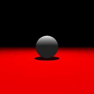
And here’s an image of a reflective red plane with a glass sphere (which really doesn’t look much like glass) on it:
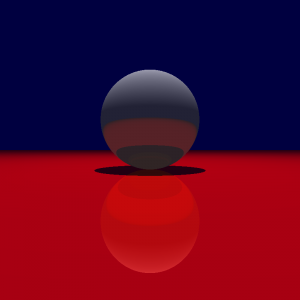
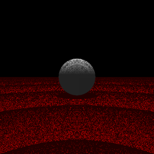
A reflective transparent sphere sitting on a reflective plane.


30
Jan 11

Ray Tracing: Shadows

Shadows are the first place where ray tracing has an advantage pipelined graphics (OpenGL). Not that shadows in pipelined graphics are impossible, but they can be a bit of a struggle (or at least they have been for me.) But as we’ll see: with ray tracing they’re actually quite pleasant.

We actually already have everything we need with the castback idea; we just need to extend them a bit so that we give shaders empty castbacks when the path to the light is blocked. What’s great is that we already have exactly that function built in, it’s the same function we use to intersect the scene. Here’s what the castback construction code looks like:

light_castback :: Scene -> Intersection -> Light -> Light_Castback
light_castback scene (Intersection _ inter_loc _ _ _) (Point light_loc color intensity) =
    if ((miss scene_xn) || light_t < (t scene_xn))
    then (Light_Castback (light_loc <-> inter_loc) color intensity)
    else empty_light_castback
 
    where ray = (ray_from_to inter_loc light_loc)
          scene_xn = (intersect_scene scene ray) --intersection with the scene
          light_dir = (light_loc <-> inter_loc)
          light_t = (len light_dir) --parameter at which we hit the light

Simple enough: we intersect with the scene and if the intersection is closer the to castbacks origin than the light we’re aiming at, we have an empty castback. So let’s see how it works:

Something is very wrong.

Hmm, not so well at all, although that is a cool looking bug. This type of effect is generally called surface acne and it’s normally down to a floating point error somewhere. In this case the problem is that the castback ray that I shoot out is, depending on roundoff errors, hitting or missing the object whose illumination we’re computing (the object it originally hit.) The easiest way to solve this is to just nudge the ray’s origin points off of the objects they’re intersecting using a function like this:

epsilon = (10 ** (-4))
 
nudge :: Ray -> Ray
nudge ray = (Ray (ray `at` epsilon) (dir ray))

Bug fixed.


24
Jan 11

Ray Tracer: Lighting (Part 1)

Up until now I’ve been cheating in creating images (although cheating is really the point of graphics). As we all know there can be no images without light so let’s add some. First off we need a few structures to represent our lights:

data Light = Point {loc :: Vec3f, 
                    color :: Color, 
                    intensity :: Float} |
             Spot {loc :: Vec3f, 
                   look_at :: Vec3f, 
                   color :: Color, 
                   angle :: Float, 
                   intensity :: Float} deriving (Show)

A point light is the simplest light, it simply shines light in every direction from a single point. A spot light is a little more complicated: it shines light in a cone (like a spotlight).

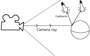
So now what can we do with these things? In an ideal world we would do with them exactly what the real world does with them: We would simulate lightrays spraying out of them bouncing around the scene and eventually entering our simulated camera. However a randomly shot lightray has a very small chance of making it to the camera so it’s computationally infeasible to start from the lights and make our way to the cameras. So we do exactly the opposite, we start from the Camera and anytime we hit a solid we try to find the lights that this ray could have started from. And we call what we find “Light castbacks”

Where castbacks come from

Light castbacks are an extra piece of information that we can pass in to our shaders; they look like this:

data Light_Castback = Light_Castback {dir :: Vec3f, 
                                      color :: Color, 
                                      intensity :: Float} deriving (Show)

With these things we have everything we need to implement some basic lighting. Here’s what the shader looks like:

shader_lit :: Shader
shader_lit (Ray_Path (Intersection _ _ norm _ False) cbs) = ((clamp 0 255 (floor (220 * foldr (+) 0 (map (\x -> (normed norm) <.> (normed (dir x))) cbs)))) <*> (1,1,1)) <+> (35,35,35)

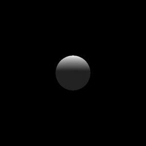
What this does is take all the castbacks from the scene and compute the dot product of the direction of the light and the normal of the surface (clamping it to within an acceptable range and boosting it to a minimum (hacky way to make there be some ambient lighting.) The fruits:

Diffuse Lighting


18
Jan 11

Ray Tracer: Shaders

Now that we can get intersections from our solids, we’re almost ready to start producing some images. We still need two things: first we need a little bit more information about the surrounding world and second we need a way to convert this information to color.

For the more information we’ll introduce a Ray_Path which looks like this:

data Ray_Path = Ray_Path {hit :: Maybe Intersection, light_hits :: [Light_Castback], shader :: Shader}

A Ray_Path gives us everything we need to understand how a ray travelled through our scene (things will have to be added to what we have right now) and convert that to color. The hit field is just an intersection from the previous post. The light_hits contain Light_Castbacks which I’m not going to define just yet–they’ll be covered in a post called “Lighting”–for now let it suffice to say that a Light_Castback will tell you everything you need to know about how this ray interacted with the lights in the scene. However we are going to talk about the shader. Shaders are the second thing we need, they’re a way to convert a Ray_Path into color. In case you don’t trust me, here’s the type signature:

type Shader = Ray_Path -> Color

Shaders are a pretty pervasive idea in graphics, and eventually I’m going to implement a full blown shader language. However for right now they’re just described in terms of a Haskell function.

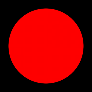
This is all we need to start doing some really simple ray tracing, so here it is: this is a simple scene with a single sphere and a shader attached to it that always returns red. Nothing too fancy, but it proves that everything underneath the hood is working:

The first render.


18
Jan 11

Ray Tracer: Geometry

The first thing we’re going to need is some geometry to shoot our rays at:

class Solid a where
    intersect :: Ray -> a -> Maybe Intersection

Basically something is a solid if we can shoot rays at it and possibly get back an Intersection (we may miss and not get back an intersection).

An Intersection is just what a record of a Ray hitting a Solid, defined as:

data Intersection = Intersection {t :: Float, loc :: Vec3f, normal :: Vec3f} deriving (Show)

Right now it only records the parameter of the ray, the location of the intersection and the normal. We’re going to need to extend that to get more sophisticated effects but we can get some simple stuff going with this.

Now that we have that we can implement our first actual primitive solid, a sphere:

data Sphere = Sphere Vec3f Float deriving (Show)
 
instance Solid Sphere where
    intersect (Ray p0 d) (Sphere c r) = case t of
        Nothing -> Nothing
        Just s -> Just (Intersection s pt (normed (pt <-> c)))
            where pt = (at (Ray p0 d) s)
        where t = (min_over_zero (real_quadratic (d <.> d) ((2 <*> d) <.> (p0 <-> c)) (((p0 <-> c) <.> (p0 <-> c)) - r ^ 2)))

15
Jan 11

Ray Tracer: Vector Module

The is going to be some of the most used code and it’s going to be a hot spot for bugs. A nice thing that Haskell does is make it very easy to define your own infix operators this should help a lot to keep things readable. Here’s the code:

module Vector (Vec3f, Color, (<+>), (<->), (<*>), (</>), (<.>), x, len, normed, Ray(Ray), at) where
 
--general purpose 3 field vector
type Vec3 a = (a, a, a)
 
(<+>) :: (Num a) => Vec3 a -> Vec3 a -> Vec3 a
(<+>) (x1,y1,z1) (x2,y2,z2) = (x1 + x2, y1 + y2, z1 + z2) 
 
(<->) :: (Num a) => Vec3 a -> Vec3 a -> Vec3 a
(<->) (x1,y1,z1) (x2,y2,z2) = (x1 - x2, y1 - y2, z1 - z2) 
 
(<*>) :: (Num a) => a -> Vec3 a -> Vec3 a
(<*>) r (x,y,z) = (r * x, r * y, r * z)
 
(</>) :: (Fractional a) => Vec3 a -> a -> Vec3 a
(</>) (x,y,z) r = (x / r, y / r, z / r)
 
(<.>) :: (Num a) => Vec3 a -> Vec3 a -> a
(<.>) (x1,y1,z1) (x2,y2,z2) = (x1 * x2) + (y1 * y2) + (z1 * z2) 
 
--cross product
x :: (Num a) => Vec3 a -> Vec3 a -> Vec3 a
x (x1,y1,z1) (x2,y2,z2) = ((y1 * z2 - y2 * z1), (x1*z2 - x2*z1), (x1 * y2 - y1 * x2))
 
len :: (Floating a) => Vec3 a -> a
len v = sqrt (v <.> v)
 
normed :: (Floating a) => Vec3 a -> Vec3 a
normed v = v </> len v
 
type Vec3f = (Vec3 Float)
type Color = (Vec3 Int)
 
--Rays
data Ray = Ray {orig :: Vec3f,
                  dir  :: Vec3f
                 } deriving (Show)
 
at::Ray -> Float -> Vec3 Float
at (Ray orig dir) t = orig <+> (t <*> dir)

Pretty basic so far, but this should be enough to get me started. Haskell wasn’t happy when I tried to make the infix operators without the “<>“s so I guess I’m stuck with them (unless someone can tell me how to fix it.) However this does still look pretty nice:

*Vector> (1,1,1) <+> (5,5,5)
(6,6,6)
*Vector> (1,1,1) <-> (5,5,5)
(-4,-4,-4)
*Vector> 5 <*> (1,2,3)
(5,10,15)
*Vector> (1,2,3) </> 5
(0.2,0.4,0.6)
*Vector> (1,2,3) <.> (3,2,1)
10
*Vector> (1,0,0) `x` (0,1,0)
(0,0,1)
*Vector> len (1,1,0)
1.4142135623730951
*Vector> sqrt 2
1.4142135623730951
*Vector> normed (1,2,3)
(0.2672612419124244,0.5345224838248488,0.8017837257372732)
*Vector> len (normed (1,2,3))
1.0
*Vector> (Ray (0,0,0) (4,3,2)) `at` 100
(400.0,300.0,200.0)

25
Aug 10

Multi Slicing

Article available at: http://www.rethinkdb.com/blog/2010/08/multi-slicing/


14
Mar 10

How Enrico Fermi Takes Integrals

You know those interview questions? The ones where you’re supposed to make spurious assumptions and use them to compute something like: “How many piano tuners are there in Chicago?”
The correct term for one of these is a “Fermi Problem” after Enrico Fermi the physicist, who apparently was spectacularly good at such problems.
Legend has it he made a stunningly accurate guess at the power of a Nuclear Explosion based on how far some nearby scraps of paper moved.

The point of Fermi Problems—and the reason they’re so popular in interviews—is to find the quickest possible path to an answer.
Even if the answer itself isn’t close enough to be useful the intuition it gives you is.
And Fermi had a great love for finding this intuition in a problem.

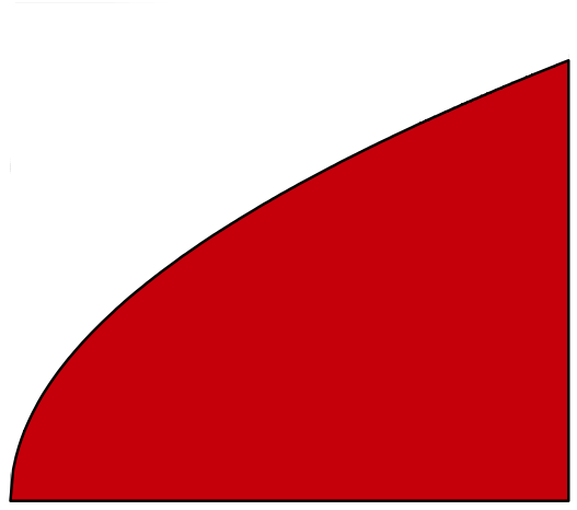
Square Root

Integration is one of the most deceptively intuitive problems out there, in the picture above for example the answer is just the red.
This easy to digest definition is what you get in the first 5 minutes of a calculus class, and then the other 1795 minutes everything is complicated and unrelated to the red.
And integrals aren’t just hard for you, it really doesn’t take much to make an integral impossible for everyone.
For example \int \sin(x)^{\sin(x)} \ dx gets you a forlorn “no result found in terms of standard mathematical functions” from Wolfram Alpha. Math just doesn’t have a good answer for it.

But this shouldn’t sit well with any of us because you know, and I know that that function has some red under it.
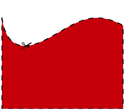
And it really didn’t sit well with Fermi so here’s what he’d do: he’d draw the function out with pencil and paper, cut it out and then weigh it.
Divide that weight by that of a 1 by 1 square of the same paper and that’s the answer.
All he needed was the first 5 minutes.

Sin(x)^Sin(x)


16
Oct 09

Programming Praxis Growable Arrays

Exercise from: http://programmingpraxis.com/2009/10/16/growable-arrays/

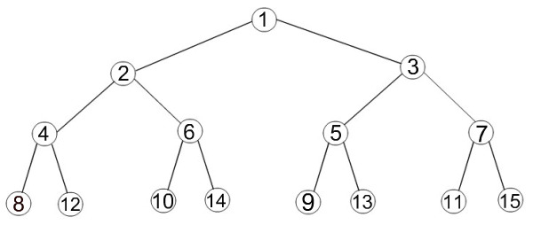
Our goal here is to implement an array which is capable of dynamically growing as we add elements to it at the cost of logarithmic runtime for put and get functions instead of the constant runtime of standard arrays. growable_arrays

The indexing scheme seems a bit weird at first until we notice the pattern that the left subtree of 1 is all even and the right subtree is all odd. So given and index we simply consider its parity and choose the correct subtree. Then we apply this recursively to the subtree with the index halved (rounded down). Here it is implemented in python:

class exArray():
	key = None
	left = None
	right = None
	def get(self, index):
		if (index == 0):
			print 'index out of bounds'
		elif (index == 1):
			if (self.key == None):
				print 'index out of bounds'
			else:
				return self.key
		elif (index%2 == 0):
			if (self.left):
				return self.left.get(index &gt;&gt; 1)
			else:
				print 'index out of bounds'
		else:
			if (self.right):
				return self.right.get(index &gt;&gt; 1)
			else:
				print 'index out of bounds'
	def put(self, index, key):
		if (index == 0):
			print 'index out of bounds'
		elif (index == 1):
			self.key = key
		elif (index%2 == 0):
			if (not self.left):
				self.left = exArray()
			self.left.put(index &gt;&gt; 1, key)
		else:
			if (not self.right):
				self.right = exArray()
			self.right.put(index &gt;&gt; 1, key)

Full code: exArray.py
To use:

import exArray
exArray.test(array_size)

29
Aug 09

The Netflix Zen Master Revisited

I was recently forwarded the response of the Netflix Zenmaster himself to my article about him. There were a few charming details I thought I might share with you. Apparently what I published was actually yesterday’s story. The Zenmaster has upped his game quite a bit since then. Nowadays content is stored on a 8TB file server he has setup in his home and streamed via wireless to all the computers and TVs in the house. It even allows for remote access through FTP. Here’s the truly golden bit: the movies have been edited to what they should have been. Annoying actors are completely edited out. As are superfluous scenes. Endings in particular are improved by this process. An example: his version of The Lord of the Rings has Frodo and Sam completely erased.